The confusion matrix is one of the most powerful tools for predictive analysis in machine learning. A confusion matrix gives you information about how your machine classifier has performed, pitting properly classified examples against misclassified examples.
Let’s take a look at how to interpret a confusion matrix and how a confusion matrix can be implemented in Scikit-learn for Python.
What Is a Confusion Matrix?
Perhaps you are wondering: What exactly is a “confusion matrix”?
Put simply, a confusion matrix is a tool for predictive analysis. It’s a table that compares predicted values with actual values. In the machine learning context, a confusion matrix is a metric used to quantify the performance of a machine learning classifier. The confusion matrix is used when there are two or more classes as the output of the classifier.
Confusion matrices are used to visualize important predictive analytics like recall, specificity, accuracy, and precision. Confusion matrices are useful because they give direct comparisons of values like True Positives, False Positives, True Negatives and False Negatives. In contrast, other machine learning classification metrics like “Accuracy” give less useful information, as Accuracy is simply the difference between correct predictions divided by the total number of predictions.
Defining Necessary Terms
Before we go any further, let's take a moment to define some important terms related to machine learning classification and predictive analytics.
Machine Learning Classification
Classification is a type of supervised learning task in the field of machine learning. The purpose of classification is to take in data points that have some number of the relevant features and use these features to predict what class, out of the chosen classes of interest, the example belongs to.
Classification tasks can be either binary in nature, with just one or two classes, or multi-class. Examples of classification problems include speech recognition (a binary problem: either speech or non-speech), document classification, diagnosing medical symptoms, and spam recognition.
True/False Positive/Negative
All estimation parameters of the confusion matrix are based on 4 basic inputs namely True Positive, False Positive, True Negative and False Negative. In order to understand what they are, let’s look at a binary-classification problem.
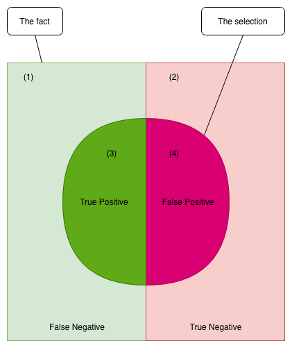
In the graphic below, we have a dataset with pre-chosen labels Positive (light green) and Negative (light red). Because the examples in the square area are based on the fact, we call it “The fact.” On the other hand, we are trying to learn a classification model for “The fact” by predicting the label of “The fact” via its features. Let’s define “The selection” as our predictions that we predict them as positive labels, represented as a circle inside the square. Obviously, the area outside the circle is the predictions which we predict negative labels.
True/False is used to describe our predictions with “The fact.” If a prediction conforms with the label it was chosen in “The fact,” it will be true, otherwise, it will be false.
Let’s take a deep look at area (1) in figure 1. Because this area was positive in “The fact,” but we predicted it negative so we got a false prediction. Thus, it is a False Negative (False means we were incorrect, Negative is from our predictions).
Similarly, area (2) is negative in “The fact” and also negative in our predictions, which makes it a True Negative. Likewise, area (3) is True Positive and area (4) is False Positive.
Recall
The term recall refers to the proportion of genuine positive examples that a predictive model has identified. To put that another way, it is the number of true positive examples divided by the total number of positive examples and false negatives.
Recall is the percentage of positive examples, from your entire set of positive examples, your model was able to identify. Recall is also sometimes called the hit rate, while sensitivity describes a model's true positive prediction rate or the recall likelihood.
Precision
Precision is similar to recall, in the respect that it’s concerned with your model’s predictions of positive examples. However, precision measures something a little different.
Precision is interested in the number of genuinely positive examples your model identified against all the examples it labeled positive. Mathematically, it is the number of true positives divided by the true positives plus the false positives.
If the distinction between recall and precision is still a little fuzzy to you, just think of it like this:
Precision answers this question: What percentage of all chosen positive examples is genuinely positive?
Recall answers this question: What percentage of all total positive examples in your dataset did your model identify?
Specificity
If sensitivity/recall is concerned with the true positive rate, specificity is concerned with tracking the true negative rate.
Specificity is the number of genuinely negative examples your model identified divided by total negative examples in dataset. It is mathematically defined by the proportion of true negative examples to true negative and false positive examples.
Accuracy
Accuracy is the simplest. It defines your total number of true predictions in total dataset. It is represented by the equation of true positive and true negative examples divided by true positive, false positive, true negative and false negative examples.
Understanding the Confusion Matrix
Now that we’ve covered the definitions of key concepts like classification, accuracy, specificity, recall, and precision, we can see how these concepts come together in a confusion matrix.
A confusion matrix is used for classification tasks where the output of the algorithm is in two or more classes. While confusion matrices can be as wide and tall as the chosen number of classes, we’ll keep things simple for now and just look at a confusion matrix for a binary classification task, a 2 x 2 confusion matrix.
Let’s say that our classifier wants to predict if a patient has a given disease, based upon the symptoms (the features) fed into the classifier. This is a binary classification task, so the patient either has the disease or they don’t.
The left-hand side of the confusion matrix displays the class predicted by the classifier. Meanwhile, the top row of the matrix stores the actual class labels of the examples.
| Prediction\Fact | Positive | Negative |
| Positive | True Positive | False Positive |
| Negative | False Negative | True Negative |
You can look at where the values intersect to see how the network performed. The number of correct positive predictions (True Positives) is located in the upper left corner.
Meanwhile, if the classifier called is positive, but the example was actually negative, this is a false positive and it is found in the upper right corner.
The lower-left corner stores the number of examples classified as negative but were actually positive, and finally the lower right corner stores the number of genuinely false examples or True Negatives.
Just to make this more explicit:
Upper Left: True Positives
Upper RIght: False Positives
Lower Left: False Negatives
Lower Right: True Negatives
If there are more than two classes, the matrix just grows by the respective number of classes. For instance, if there are four classes it would be a 4 x 4 matrix.
No matter the number of classes, the principal is still the same: The left-hand side is the predicted values and the top the actual values. Just check where they intersect to see the number of predicted examples for any given class against the actual number of examples for that class.
You should also note that the instances of correct predictions will run down a diagonal from top-left to bottom-right. From seeing this matrix you can calculate the four predictive metrics: sensitivity, specificity, recall, and precision.
For example,

While you could manually calculate metrics like precision and recall, these values are so common in predictive analysis that most machine learning libraries, such as Scikit-learn for Python, have built-in methods to get these metrics.
Generating A Confusion Matrix In Scikit Learn
So how do you generate a confusion matrix for a machine learning task? We’ve covered the theory behind a confusion matrix, so now let’s go over an example of implementation.
This example will cover implementing a confusion matrix in Scikit-learn (Sklearn). Seeing how confusion matrices are generated in practice will help you understand their intended use.
To start with, we need to decide on a dataset to use for analysis. For this example, we will be using the “digits” data set.
The digits dataset is a collection of handwritten numbers, and our classifier will try to predict which number is in a given example. It comes pre-packaged into Scikit-learn, and because of the fact that the data set is so well-maintained, very little preprocessing of the data is necessary.
Let's begin by importing the necessary modules into Python. We will be using Scikit-learn, as previously mentioned.
We'll need the logistic regression classifier, the train/test split tool, and the confusion matrix metric from Sklearn. We will also be making use of Numpy and Matplotlib.
Numpy is used to transform the data into a type usable by our classifier, while Matplotlib is used to visualize the data.
import numpy as np
import matplotlib.pyplot as plt
from sklearn.metrics import confusion_matrix
from sklearn.linear_model import LogisticRegression
from sklearn.model_selection import train_test_split
Now that we have important the necessary modules, let's load in the dataset.
from sklearn.datasets import load_digits
digits = load_digits()
Let's visualize some of the data using matplotlib to make sure the data has been loaded correctly.
plt.figure(figsize=(20,4))
for index, (image, label) in enumerate(zip(digits.data[0:5], digits.target[0:5])):
plt.subplot(1, 5, index + 1)
plt.imshow(np.reshape(image, (8,8)), cmap=plt.cm.gray)
plt.title('Training: %i\n' % label, fontsize = 20)
Now we need to split our data up into a training set and testing site, as well as features and labels. The "X"s are the features, while the "Y"s are the labels.
X_train, X_test, y_train, y_test = train_test_split(digits.data, digits.target, test_size=0.25, random_state=0)
Now we need to create an instance of our classifier. We will be using the logistic regression classifier, which we have previously imported.
logreg_clf = LogisticRegression()
After creating an instance of the classifier, we can fit the classifier and have it train on the data simply by calling the "fit" command on it.
logreg_clf.fit(X_train, y_train)
Now that we have a fitted classifier, we can pass it images to classify. We can give it either a single image at a time, or multiple images by slicing that the data set.
# How to predict a single example
logreg_clf.predict(X_test[0].reshape(1,-1))
# How to predict multiple examples, by slicing the dataset
logreg_clf.predict(X_test[0:10])
Now let's make predictions out of the entire test data set, bypassing it the "X_test" variable. We will also store the predictions in a variable called "predictions" so we can access them when evaluating the performance of the classifier.
predictions = logreg_clf.predict(X_test)
Now, all we have to do is evaluate our classifier’s performance. We can do this by simply calling the "score" command on the logistic regression object to get a quick idea of the classifier's accuracy.
However, to get the confusion matrix for our classifier, we need to create an instance of the confusion matrix we imported from Sklearn and pass it the relevant arguments: the true values and our predictions.
score = logreg_clf.score(X_test, y_test)
print(score)
c_matrix = confusion_matrx(y_test, predictions)
print(c_matrix)
That's how you generate a confusion matrix in Sklearn. There are other ways to generate a confusion matrix in Python as well, such as by using the Seaborn library, but this is one of the simplest ways to do it.
Conclusion
A confusion matrix is a powerful tool for predictive analysis, enabling you to visualize predicted values against actual values. It will take some time to get used to interpreting a confusion matrix, but once you have done so it will be an important part of your toolkit as a data scientist.
You will also want to learn about the other forms of model evaluation for machine learning systems, just be sure to keep the usefulness of confusion matrices in mind.
Vietnam AI Grand Challenge Community Voting Begins!

Across Vietnam, Kambria has been working with young developers utilizing machine learning principles like the confusion matrix to develop innovative AI solutions.
Held in collaboration with the Vietnamese government, McKinsey & Company, and VietAI, the Vietnam AI Grand Challenge is bringing together the country’s best AI talent to design the Ultimate AI Virtual Assistant. Design sectors include self-driving cars, manufacturing, banking, hotel services, and more. In total, 187 teams signed up with over 700 participants!
Community voting is now open. We invite you to participate in shaping the outcome of the Challenge and to support all of the amazing teams. The two teams with the most Community Votes and with at least 200 votes will receive free airfare and accommodation to compete in the Grand Finale in Hanoi on August 15th as part of the AI4VN program.
Anyone can vote! Voting is free! As an added bonus, everyone who votes will be entered into a giveaway. Read our full blog post here for all of the details.
Vote Now!


